
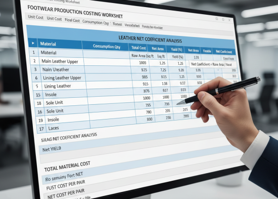
Footwear Manufacturing Cutting-2 : Calculating True Leather Cost Using Cuttable Area
Estimated Reading Time: ~ 5 minutes
Introduction
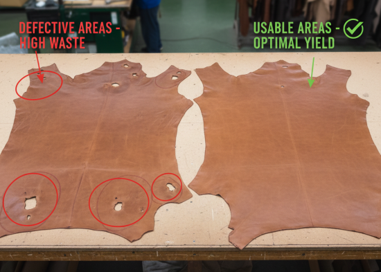
In footwear manufacturing, leather is usually purchased based on gross area declared by the vendor. However, only a portion of this area is actually usable for cutting shoe components. Defects, shape limitations, and area discrepancy reduce the effective yield. Therefore, the true cost of leather cannot be evaluated using purchase price alone.
This section explains how to calculate the cost per cuttable square foot, using the net coefficient, and how this data is further used to analyze purchase cost variance.

1. Why Purchase Price Alone Is Misleading
Leather with a lower purchase price may appear economical. However:
- High defect levels reduce usable area
- Poor cuttability increases waste
- Area shortfall increases effective cost
As a result, two leathers with the same purchase price may have very different true costs when converted into shoe components.
The solution is to calculate the cost of cuttable area, which reflects the real material cost used in production.
2. Net Coefficient as the Costing Base
The Net Coefficient (G) represents the combined effect of:
Net Coefficient G = E * F
E = Area discrepancy coefficient of the sample
F = Cuttability coefficient of the sample
This coefficient must always be used as the base for leather cost calculations.

3. Cost per Cuttable Square Foot
3.1 Objective
The objective is to convert the purchase price per square foot into the actual cost per usable square foot. Defective leather area has no cutting value. Therefore, the true leather cost is the cost of the cuttable area only.
3.2 Cost Formula
Cost per Cuttabe Sq.ft I = H/G
H =Purchase Price sq.foot ,as state by the vendor
G= Net Coefficeint
3.3 Leather Cost per Cuttable Area
Table 2 – Leather Cost per Cuttable Square Foot
| Receipt | E | F | G | H | I | |||
| PO# & Date | Thickness | Color | Grade | Area discr. Coeff. | Cuttability coefficient | Net Coeff G = E*F | Purchase Price /Sq.ft | Cost per cuttable sq.ft I = H/G |
| 001 1-Jan | 1.6 – 1.8 | Black | A | 0.94 | 0.97 | 0.91 | 2.66 | 2.92 |
| B | 0.95 | 0.88 | 0.84 | 2.54 | 3.02 | |||
| C | 0.94 | 0.88 | 0.77 | 2.41 | 3.13 | |||
| D | 0.94 | 0.79 | 0.74 | 2.30 | 3.11 | |||
| 002 10-Jan | 1.8 – 2.0 | Black | A | 0.93 | 0.92 | 0.86 | 2.66 | 3.24 |
| B | 0.94 | 0.84 | 0.79 | 2.54 | 3.22 | |||
| C | 0.93 | 0.80 | 0.74 | 2.41 | 3.24 | |||
| D | 0.92 | 0.80 | 0.74 | 2.30 | 3.13 | |||
This table clearly shows that lower-grade leather may have a higher effective cost, despite a lower purchase price.

4. Setting Standard Net Coefficients
4.1 Purpose of Standards
Standards are required to:
- Evaluate vendor performance
- Compare actual results with expectations
- Control leather purchasing decisions
Standard net coefficients are future-oriented estimates derived from historical data.
4.2 Example: Standard Net Coefficient by Grade
| Grade of Leather | Standard Area Coefficient | Standard Cuttability Coefficient | Standard Net Coefficient | Std. Mix of Grades (Ratio) | Breakdown of Mix |
| A | 0.98 | * 0.94 | = 0.92 | *0.10 | = 0.092 |
| B | 0.98 | * 0.88 | = 0.85 | *0.40 | = 0.344 |
| C | 0.98 | * 0.83 | = 0.81 | *0.40 | = 0.324 |
| D | 0.98 | * 0.78 | = 0.76 | *0.10 | = 0.076 |
| Std. Weighed Average Net Coefficient | 0.836 | ||||
5. Standard Cost per Cuttable Square Foot
5.1 Calculation Logic
Standard cost is calculated using:
- Standard net coefficient
- Standard purchase price
5.2 Example: Standard Cost Calculation
| Grade of Leather | Standard Area Purchase Price | Standard Net Coefficient | Standard cost per cuttable sq.ft | Std.mix of grades (ratio) | Breakdown of Std units |
| A | 2.71 | ÷ 0.92 | = 2.95 | *0.10 | = 0.230 |
| B | 2.59 | ÷ 0.81 | = 3.01 | *0.40 | = 1.254 |
| C | 2.46 | ÷ 0.81 | = 3.04 | *0.40 | = 1.216 |
| D | 2.35 | ÷ 0.76 | = 3.09 | *0.10 | = 0.309 |
| Std. cost per cuttable Sq.ft (J) | 3.02 | ||||

6. Purchase Cost Variance of Leather
6.1 Objective
Purchase cost variance measures:
- Deviation from established standards
- Vendor performance
- Purchasing efficiency
6.2 Variance Formula
Purchase cost variance of leather N = (K*J)-L
J = Standard unit cost per cuttable Sq.foot
K = Total quantity received, measured by the Vendee
L = Cost of total Received cuttable Area
6.3 Example: Actual Performance Analysis
| Grade of Leather | Actual Purchase Price H | Net Coefficient G | Actual Cost Per Cuttable Sq.ft I | Recd Qty in Sq.ft K | Cost of Received Cuttable Area L |
| A | 2.66 | ÷ 0.91 | = 2.92 | * 105 | = 306.60 |
| B | 2.54 | ÷ 0.84 | = 3.02 | *430 | = 1298.60 |
| C | 2.41 | ÷ 0.77 | = 3.13 | *385 | = 1205.60 |
| D | 2.30 | ÷ 0.74 | = 3.11 | *80 | = 248.80 |
| L = Cost of total Received cutting area K = Total Received Qty N = Purchase cost Variance = (K*J) – L = (1000*3.02) – 3059.60 | 3059.60 1000. Sq,ft – 39.60 Favorable (+) Unfavorable (-) | ||||
7. Using Purchase Variance for Management Control
Purchase cost variance data can be:
- Cumulated by leather type
- Analyzed by vendor
- Used for negotiation and sourcing decisions
Table 3 – Summary of Purchase Cost Variance (Conceptual)
This summary helps management identify long-term trends rather than isolated shipment issues.
| K | M | N | |||||
| PO# Date | Vendor | Qty Received (Sq.ft) | Standard Cost of cuttable Area K*J | Purchase Variance Cost (N*100) /M | % | Cumulative purchase cost variance (Cumul.N) *100 /Cumul.M | % |
Conclusion
Calculating leather cost based on cuttable area transforms leather purchasing from a price-based decision into a performance-based system. By applying net coefficients, setting standards, and analyzing purchase cost variance, footwear factories gain transparency and control over one of their most critical cost elements.